The coherent gain of a window a(k) of length N is
$$CG=\frac{1}{N} \sum_{k=0}^{N-1} a(k)$$
As computed, this coherent gain is normalized by the length of the window N.
Example of the application of the coherent gain
Consider the example signal x(k) with frequency 60 Hz over the sampling frequency 400 Hz.
$$x(k)=\sin(\frac{2\pi k \,60}{400})$$
Suppose that we use the discrete Fourier transform of 20 components to compute the magnitude |H(m)| of the frequencies 0 Hz, 20 Hz,…, 380 Hz in this signal.
$$H(m)=\sum_{k=0}^{M-1} x(k) e^{-\frac{2\pi\,j\,k\,m}{N}}$$ $$=\sum_{k=0}^{M-1} x(k) \cos(\frac{2\pi\,k\,m}{N})-j \sum_{k=0}^{M-1} x(k) \sin(\frac{2\pi\,k\,m}{N})$$ $$|H(m)|=\sqrt{(Re(H(m)))^2+(Im(H(m)))^2}$$
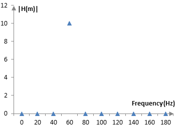
M = 20, m = 0, 1, …, M – 1. The magnitude of 60 Hz in x(k) will be computed as 10, whereas the magnitude of the remaining frequencies will be approximately zero. This is so as the frequency 60 Hz is a multiple of the Fourier transform step of 20 Hz and fits nicely in the first 20 samples. The computed magnitude content of x(k) is shown on the graph below.
The Fourier transform is not so precise for all frequencies. With x(k) = 55 Hz, for example, we get the following graph.
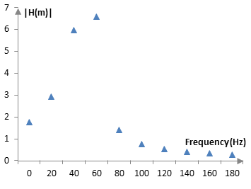
This signal does not fit nicely (does not complete an integer number of cycles) in the first 20 samples and hence its magnitude spills over into several components of the Fourier transform. There is spectral leakage.
To remedy this spectral leakage, we can apply a window to the signal x(k). The following graph shows the magnitude content of the signal, computed with the Fourier transform, before and after the Hann window is applied to the signal. The Hann window used here is of length M = 20, the length of the Fourier transform. This graph is computed with an adjustment for the coherent gain of the window, as explained below.
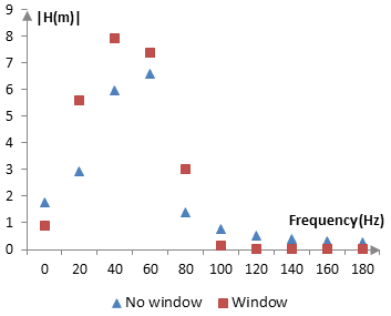
The window reduces spectral leakage, as it decreases the signal towards the two ends of the 20 samples and, hence, whether or not the signal fits nicely in the 20 samples becomes less important. In the graph above, the magnitudes with the window concentrate more around the actual frequency of the signal. The Fourier transform is more precise.
The following is the signal before and after the window.
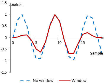
Once a window is applied to the signal, however, the magnitudes of the signal computed with the Fourier transform will decrease. The coherent gain of the window is a measure of this decrease. The magnitudes computed with the Fourier transform must be adjusted (divided) by the coherent gain to be comparable. The coherent gain of the 20-point Hann window in this example is 0.475. With larger Hann windows, the coherent gain will approach 0.5.
Similar "spectral leakage" also occurs when the discrete Fourier transform is computed at points between the actual transform components. Consider the following graph.
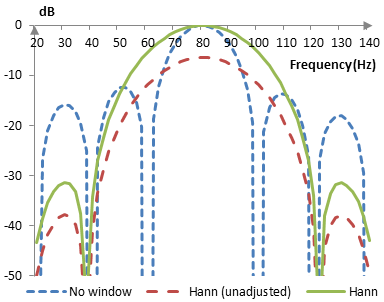
Computations, similar to those of the discrete Fourier transform, are used to analyze the frequency content of the simple sine wave at 80 Hz with and without the Hann window. The Hann window reduces spectral leakage, but the results of the Hann window have to be adjusted with the coherent gain to produce the expected amplitude of 0 dB at 80 Hz.
Coherent gain for common windows
The following is the coherent gain of some common windows (with the window definitions on this site).
| Bartlett-Hann | 0.50 |
| Blackman Exact Blackman Generalized Blackman α = 0.05 α = 0.20 α = 0.35 |
0.42 0.43 0.47 |
| Blackman-Harris | 0.36 |
| Blackman-Nuttall | 0.36 |
| Bohman | 0.40 |
| Dolph-Chebychev ω0 = 0.1 ω0 = 0.2 ω0 = 0.3 |
0.34 0.25 0.20 |
| Flat top | 0.22 |
| Gaussian σ = 0.3 σ = 0.5 σ = 0.7 Approximate confined Gaussian σ = 0.3 σ = 0.5 σ = 0.7 Generalized normal α = 2 α = 4 α = 6 |
0.37 0.60 0.74 0.37 0.60 |
| Hamming | 0.54 |
| Hann | 0.50 |
| Hann-Poisson α = 0.3 α = 0.5 α = 0.7 |
0.46 0.43 0.41 |
| Kaiser α = 0.5 α = 1.0 α = 5.0 |
0.85 0.67 0.42 |
| Kaiser-Bessel | 0.40 |
| Lanczos | 0.59 |
| Nuttall | 0.36 |
| Parzen | 0.69 |
| Planck-taper ε = 0.2 ε = 0.4 ε = 0.5 |
0.80 0.60 0.50 |
| Poisson α = 0.2 α = 0.5 α = 0.8 |
0.91 0.79 0.69 |
| Power of cosine α = 1.0 α = 2.0 α = 3.0 |
0.64 0.50 0.42 |
| Rectangular | 1.00 |
| Sine | 0.64 |
| Triangular | 0.50 |
| Tukey α = 0.3 α = 0.5 α = 0.7 |
0.65 0.75 0.85 |
| Ultraspherical (x0 = 1) μ = 2 μ = 3 μ = 4 |
0.68 0.55 0.48 |
| Welch | 0.67 |
Add new comment