The Hann window coefficients are given by the following formula
$$a(k)=0.5 * (1-\cos(\frac{2\pi\,k}{N-1}))$$
where N is the length of the filter and k = 0, 1, …, N – 1.
The Hann window belongs to the family of Hamming windows. The derivation of the Hann window is shown in the topic Hamming window. The Hann window is also a poiwer of cosine window (α = 2). When the Hann window is multiplied by the Poisson window, the result is the Hann-Poisson window.
An example Hann window
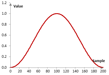
Consider a finite impulse response (FIR) low pass filter of length N = 201. The following is the Hann window.
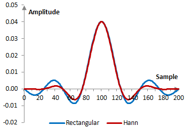
Given a sampling frequency of 2000 Hz and a filter cutoff frequency of 40 Hz, the impulse response of the filter with a rectangular window (with no window) and with the Hann window is as follows.
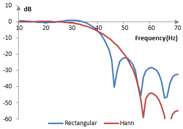
The magnitude response of the same filter is shown on the graph below.
Measures for the Hann window
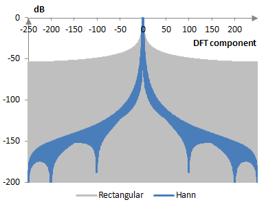
The following is a comparison of the discrete Fourier transform of the Hann window and the rectangular window.
The Hann window measures are as follows.
| Coherent gain | 0.50 |
| Equivalent noise bandwidth | 1.50 |
| Processing gain | -1.77 dB |
| Scalloping loss | -1.42 dB |
| Worst case processing loss | -3.19 dB |
| Highest sidelobe level | -31.5 dB |
| Sidelobe falloff | -20.7 dB / octave, -68.9 dB / decade |
| Main lobe is -3 dB | 1.44 bins |
| Main lobe is -6 dB | 2.00 bins |
| Overlap correlation at 50% overlap | 0.165 |
| Amplitude flatness at 50% overlap | 1.000 |
| Overlap correlation at 75% overlap | 0.658 |
| Amplitude flatness at 75% overlap | 1.000 |
See also:
Window
Add new comment