The Blackman-Nuttall window coefficients are given by the following formula
$$a(k)=0.3635819-0.4891775 \, \cos(\frac{2\pi k}{N-1})$$ $$+0.1365995 \, \cos(\frac{4\pi k}{N-1})-0.0106411 \, \cos(\frac{6\pi k}{N-1})$$
where N is the length of the filter and k = 0, 1, …, N – 1.
The Blackman-Nuttall window is a generalized cosine window (see Hamming window).
An example Blackman-Nuttall window
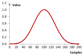
Consider a finite impulse response (FIR) low pass filter of length N = 201. The following is the Blackman-Nuttall window.
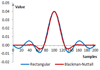
Given a sampling frequency of 2000 Hz and a filter cutoff frequency of 40 Hz, the impulse response of the filter with a rectangular window (with no window) and with the Blackman-Nuttall window is as follows.
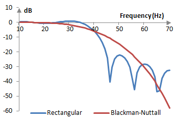
The magnitude response of the same filter is shown on the graph below.
Measures for the Blackman-Nuttall window
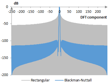
The following graph compares the discrete Fourier transform of the Blackman-Nuttall window and the rectangular window.
The Blackman-Nuttall window measures are as follows.
| Coherent gain | 0.36 |
| Equivalent noise bandwidth | 1.98 |
| Processing gain | -2.97 dB |
| Scalloping loss | -0.85 dB |
| Worst case processing loss | -3.81 dB |
| Highest sidelobe level | -98.3 dB |
| Sidelobe falloff | -12.7 dB / octave, -42.2 dB / decade |
| Main lobe is -3 dB | 1.88 bins |
| Main lobe is -6 dB | 2.62 bins |
| Overlap correlation at 50% overlap | 0.041 |
| Amplitude flatness at 50% overlap | 0.454 |
| Overlap correlation at 75% overlap | 0.469 |
| Amplitude flatness at 75% overlap | 1.000 |
See also:
Window
Add new comment